Hardware Graph Prefetchers

This week sees the publication of two papers from my research group at ICS 2016 and so, in this post, I’d like to look a little more into one of these schemes: the graph prefetcher that my student, Sam, has developed.

Graph workloads are important in a number of domains, and becoming increasingly so.  You only have to look at the numerous social media applications to see examples of graph-based data (e.g. in a network of people, each person is a vertex and the edges represent links to friends).  But graph representations are also significant in less publicly-visible application areas, such as those in scientific computing or “big data” analytics.  However, efficient processing of graph workloads is often more difficult than it might first seem.

We looked into how graph applications run on a standard Intel-based machine, shown in the figure below.  (As an aside, I’d rather refer to figures as graphs, since that’s what they are, but it’s going to get really confusing if I talk about two different kinds of graph, and I’m definitely not going to refer to them as plots, so figures is my compromise!)  In this, we plot the trend for different graph sizes using the Graph 500 benchmark.  In this workload, the scale refers to the size of the graph (there are 2 to the power scale vertices in the graph) and the edge factor refers to the ratio of edges to vertices.  Put simply, a large scale means a bigger graph, and a larger edge factor means that the graph is more connected.  The benchmark performs a breadth-first search through the graph, visiting all vertices.

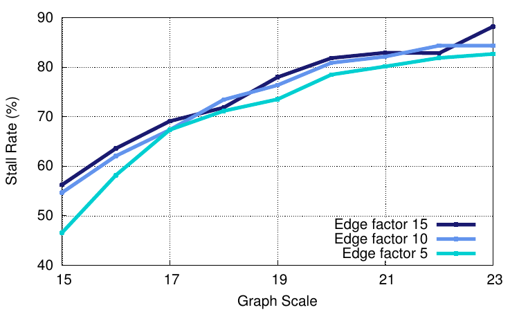As can be seen, as the graph increases in size, the amount of time the processor spends stalling also increases.  With the larger graphs, we see stall rates of over 80%.  That’s only one cycle of work out of every five, and this is for graphs that fit in main memory – imagine what would happen if they didn’t!  As we show in our paper, the reason behind this is that the L1 data cache miss rate is high – approaching 50%.  Lumsdaine et al.¹ define four properties of graph problems that make them difficult to parallelise.  These are (1) data driven computation, (2) unstructured problems, (3) poor locality, and (4) high data access to computation ratio.  Right now, we’re not too concerned with parallelising the graph computation (at least, not just yet); we just want it to be faster.  However, some of these properties (if not all) also cause problems for us.  In our example above, we are seeing the effects of poor locality (which is what the cache is designed for), combined with the high data access to computation ratio (meaning that the processor can’t do much useful work whilst waiting for data).

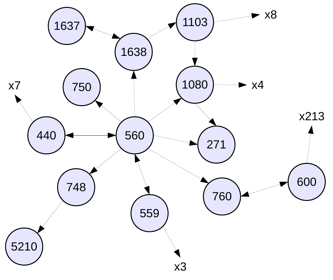What is it about these graph traversals that’s causing so many misses and so many stalls?  To answer that, I’m going to show an example graph and the start of the traversal through it.  I’m showing a real example here: part of the wiki-Vote graph from the SNAP datasets².  I would have used one from our paper, but this was considerably smaller and easier to work with for the purposes of this post.

Let’s assume we perform a breadth-first traversal of the graph, starting from node 560.  We add nodes to visit to a FIFO work list, which is implemented as an array.  This is shown below, along with three other arrays necessary for performing this traversal using the compressed sparse row format.  The vertex list is indexed by vertex number, v.  It contains the first index into the edge list for the given vertex’s edges.  The edge list stores vertex IDs in consecutive locations for each edge out of v.  To find all edges for v we must access edgeList[vertexList[v]] to edgeList[vertexList[v+1]].   The last structure is the visited list which is also indexed by vertex ID, and this contains information on whether the vertex has been seen or not.

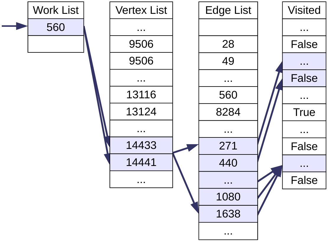So, since we are starting at vertex 560, we access the vertex list at index 560 and 561 to find the edge information.  The first of these is likely to miss in the cache, since it is unlikely that this part of the vertex list has been recently accessed.  The second will likely hit due to spatial locality because the two indices will probably be mapped to the same cache line.  We then access the edge list at indices 14433 through to 14440.  Again, the first access will likely miss, but due to spatial locality, subsequent accesses will likely hit up to the end of the cache line.  In our example, we would expect 2 misses (the first from index 14433, the second from index 14440), assuming 64 byte cache lines, 8 byte array items and an aligned array.  Finally, the visited list is accessed for each of these 8 target vertices and, since none of these vertices have been visited, they all get added to the work list.  We’d expect 7 misses here using the same assumptions as before (indices 748 and 750 should map to the same cache line), but note that the Boost Graph Library stores the visited information using just two bits per entry, meaning there is a greater chance of exploiting spatial locality with this format.

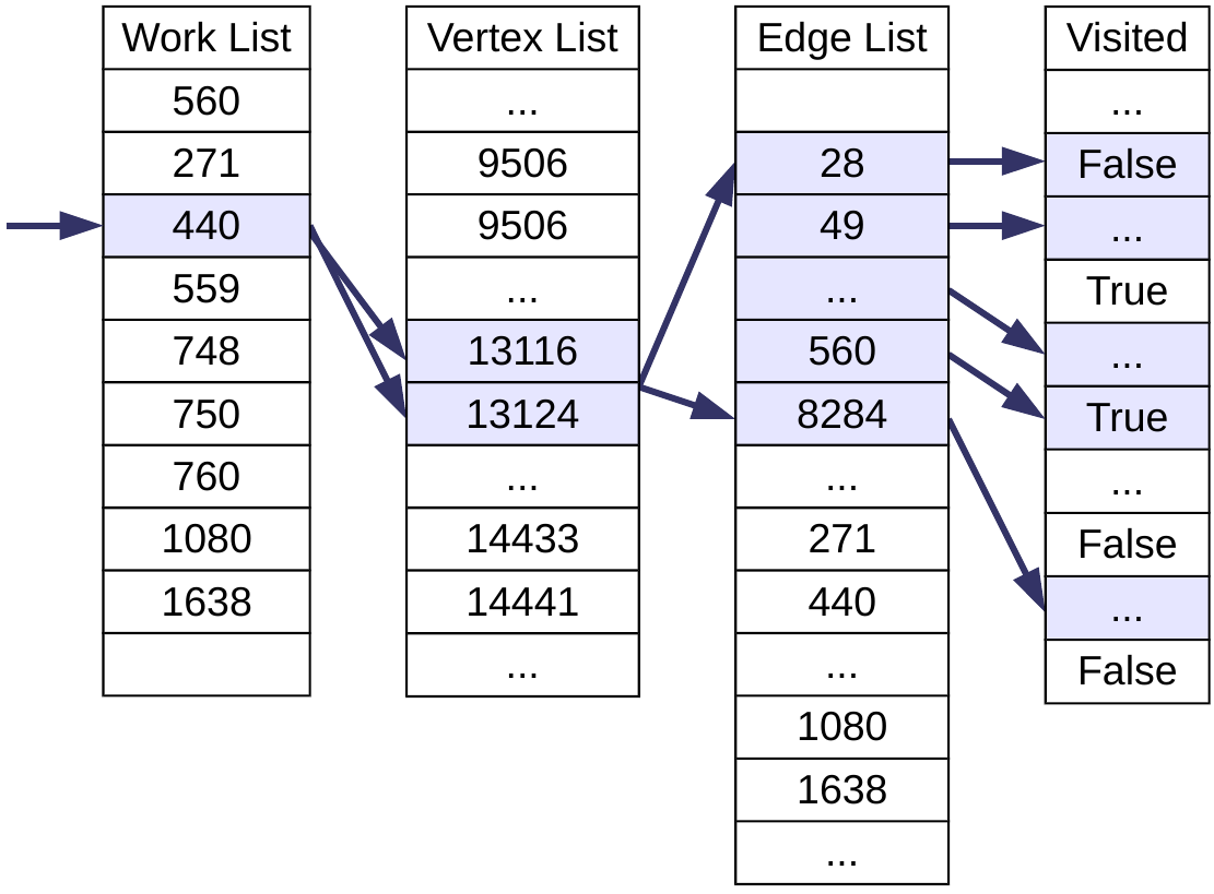Moving on, we then process the next vertex on the work list, which is 271.  Since this doesn’t have any outgoing edges, we only need to access the vertex list (another miss).  Vertex 440 is next and this has 8 outgoing edges.  This will cause 1 miss when accessing the vertex list, 2 misses accessing the edge list (because the indices cross a cache line boundary once again), and 7 misses accessing the visited list (visited information for the starting node, 560, which has an edge to and from 440, will already be in the cache).  We continue working through the graph in this manner until all vertices have been visited.

From the example above it’s clear why there is little locality within the graph computation, meaning that there’s a lot of places where the data simply won’t be in the cache and the processor must stall.  Existing hardware prefetchers can’t help here because we’re jumping all around in memory and there are seemingly no patterns in the accesses.

However, the insight in our paper is that we actually do know quite a lot about the upcoming memory accesses, simply by looking at the structures we’ve got and adding a little semantic knowledge into the hardware.  For example, we know that the work list is accessed one item after another.  We know that this contains indices into the vertex list, that only two consecutive items from this list are accessed and that these are indices into the edge list.  We know that we access a range of consecutive items from the edge list and that these are indices into the visited list.  Furthermore, we know that to process one item from the work list we traverse all of these structures (except where there are no outgoing edges from a vertex).  This means that once we have accessed the work list, we will definitely access the vertex list.  Once we have indices from there, we will use them in the edge list, and so on.  The memory accesses are structured and predictable, as long as we use information from within the data structures to help us out.

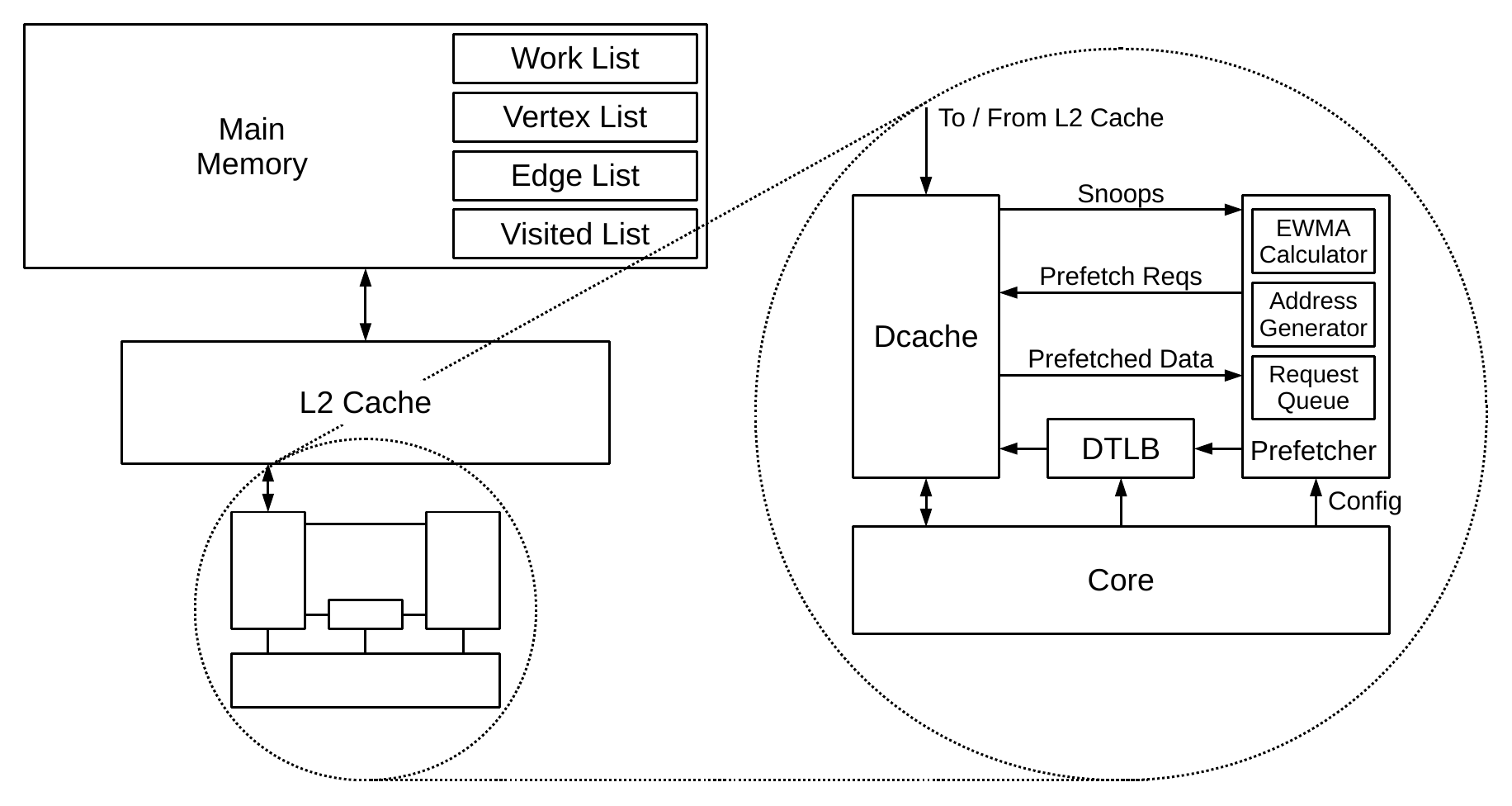This is the resulting prefetcher that we developed to speed up graph breadth-first search and similar traversals.  Like existing prefetchers, it sits beside the cache and snoops accesses to it.  Unlike existing hardware, it needs to be explicitly configured with the base and end addresses of each of the four lists that are used during the traversal.  Also novel is that it snoops prefetched data when it reaches the cache, enabling the prefetcher to create even more prefetches on the back of that.  The prefetcher works on virtual addresses, since all the lists are software constructs, so it needs access to the TLB for address translation.  Let’s look at the microarchitecture in more detail to explain how it works.

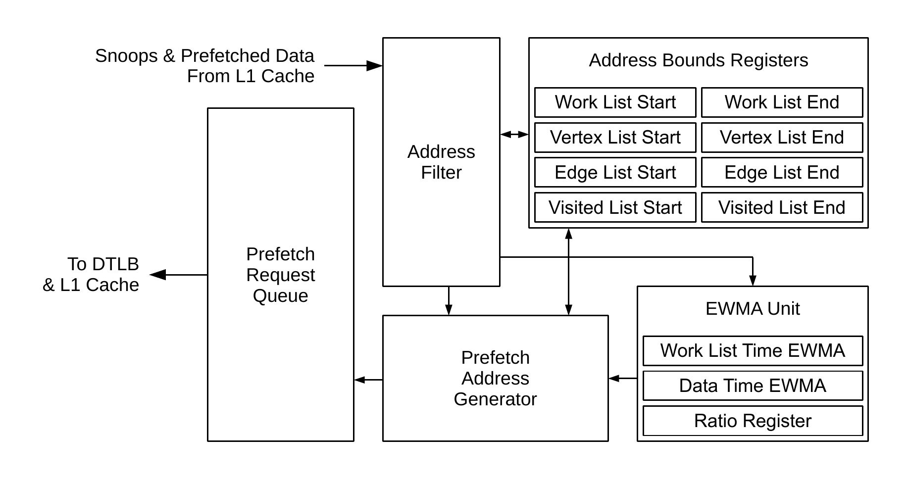Snooped loads and prefetched data enter the address filter first.  This uses the explicit list bounds registers to determine whether the access is to a structure that the prefetcher is interested in (i.e. whether it is within one of these lists).  Everything outside is ignored, which prevents the prefetcher from reacting to events that are not part of a graph traversal.

The prefetch address generator is responsible for creating new prefetches.  It uses the information about the traversal structure described above to do this.  For example, if prefetched data returns from within the vertex list, then the prefetch address generator will create prefetches into the edge list using this data.  The EWMA unit also comes into play at this point, and more of that is described below.  Prefetches are kicked off when the core accesses an item on the work list.  A load of work list item n generates a prefetch to another work list item at position n + o, where o is determined by an EWMA.  When this prefetch returns, a prefetch to the relevant vertex list entry is generated, and so on.  Prefetches themselves are placed in the prefetch request queue to be scheduled when the cache is able.

The EWMAs (exponentially weighted moving averages) are running calculations designed to estimate key values for the prefetcher that can vary by system, application and graph.  The offset to prefetch into the work list, mentioned above, relies on these values.  This offset needs to be set so that all the data for a particular vertex is available in the cache immediately before this vertex is accessed from the work list.  It varies by system (due to the memory access latency and cache hierarchy configuration), by application (according to the amount of non-traversal work performed for vertex) and by section of the graph (because some vertices contain many outgoing edges, whereas others have very few).  The paper contains more details, including the equations used.

Finally, the prefetcher has two modes of operation: vertex-offset and large-vertex modes.  Going back to the example wiki-Vote graph above helps explain why.  For the majority of vertices shown, there are a small number of outgoing edges, meaning that it doesn’t take too long to perform the traversal over these vertices when they are accessed from the work list.  This corresponds to vertex-offset mode, where we can process several vertices from the work list whilst prefetching all the data for the vertex immediately afterwards.  I.e. we need to prefetch at an offset (o > 1) from the current vertex to ensure that all data is in the cache by the time we need it.

However, other vertices have large numbers of outgoing edges (in the example graph above, vertex 600 has 213 outgoing edges, for example, but in this graph the maximum is 893).  Processing these vertices requires more time than it would take to prefetch all data from the next vertex on the work list.  In this situation, we don’t want to prefetch that next vertex too early because it is likely that its data will be evicted from the cache before it is actually used.  (A 32KiB cache contains 512 lines of 64 bytes, and assuming that none of the visited list entries map to the same cache line, then not even all data for the current vertex might fit in the L1.)  This is where large-vertex mode comes into play.  We basically stop prefetching future vertices from the work list and instead concentrate on prefetching for the current vertex.  Towards the end of computation on the current vertex’s edge list, we then start to prefetch the next work list item.

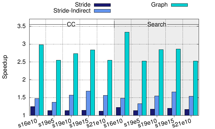So, what can our graph prefetcher actually do?  Let’s try it out on some of the graphs from the original figure at the top of this post.  Results are plotted in the figure on the right and clearly  show the benefits of embedding the structure of the graph into the hardware.  The figure on the right shows speedups for Graph 500 for varying scales and edge factors, across two algorithms (connected components and breadth-first search), but there’s much more in the paper.  Our prefetcher enables significant speedups, vastly more than two comparison techniques of a simple stride prefetcher and a recently-proposed stride-indirect prefetcher³ which do mostly increase performance, just not by very much in comparison.

So, there you have it.  We’re looking to extend this prefetcher to become more generalised and apply it to other forms of computation that are memory bound.  I believe there are a number of key applications and kernels out there that could benefit from a prefetcher with knowledge about the structures and semantics of the memory accesses and we’re going to see how much performance they can gain through a more intelligent prefetching technique.