
Submitted by Timothy Jones on Tue, 27/10/2015 - 11:25
It sounds a bit counter-intuitive, but boosting application performance by limiting the amount of vectorisation carried out is essentially what my postdoc, Vasileios Porpodas, and I have done in our latest paper on automatic vectorisation. We call it TSLP, or Throttled SLP, because it limits the amount of scalar code that the standard SLP algorithm converts into vectors.
The actual paper is available here. Vasileios presented it at PACT last week and will be at the LLVM Developers’ Meeting this week, so I thought it might be interesting to expand on one of the examples we give at the end, showing the source code and how it is actually vectorised with SLP and TSLP. The kernel is compute-rhs, which is a function from the BT benchmark within the NAS parallel benchmark suite. The code we’re interested in is this:
1:  rhs[i][j][k][2] = rhs[i][j][k][2] +
2:    dx3tx1 * (u[i+1][j][k][2] - 2.0*u[i][j][k][2] + u[i-1][j][k][2]) +
3:    xxcon2 * (vs[i+1][j][k] - 2.0*vs[i][j][k] + vs[i-1][j][k]) -
4:    tx2 * (u[i+1][j][k][2]*up1 - u[i-1][j][k][2]*um1);
5:
6:  rhs[i][j][k][3] = rhs[i][j][k][3] +
7:    dx4tx1 * (u[i+1][j][k][3] - 2.0*u[i][j][k][3] + u[i-1][j][k][3]) +
8:    xxcon2 * (ws[i+1][j][k] - 2.0*ws[i][j][k] + ws[i-1][j][k]) -
9:    tx2 * (u[i+1][j][k][3]*up1 - u[i-1][j][k][3]*um1);
Lovely, isn’t it! The code is executed in a loop nest with the outer loop using iteration variable i, the next using j and the inner loop having iteration variable k. All scalar variables are globals and, although it doesn’t matter to us, everything is a double.
Just by looking at the code, it’s obvious that there are similarities between the two statements, although they are not identical and so vectorisation isn’t trivial. Variables um1 and up1 are local to the function; all others are global. Also, because we extracted this kernel from the actual benchmark, we didn’t include the code that initialises any of the arrays.
The SLP graph created for these two statements follows. It’s just the same as figure 11(a) from our paper, but I’ve reproduced it here to save flicking back and forth between this page and that.
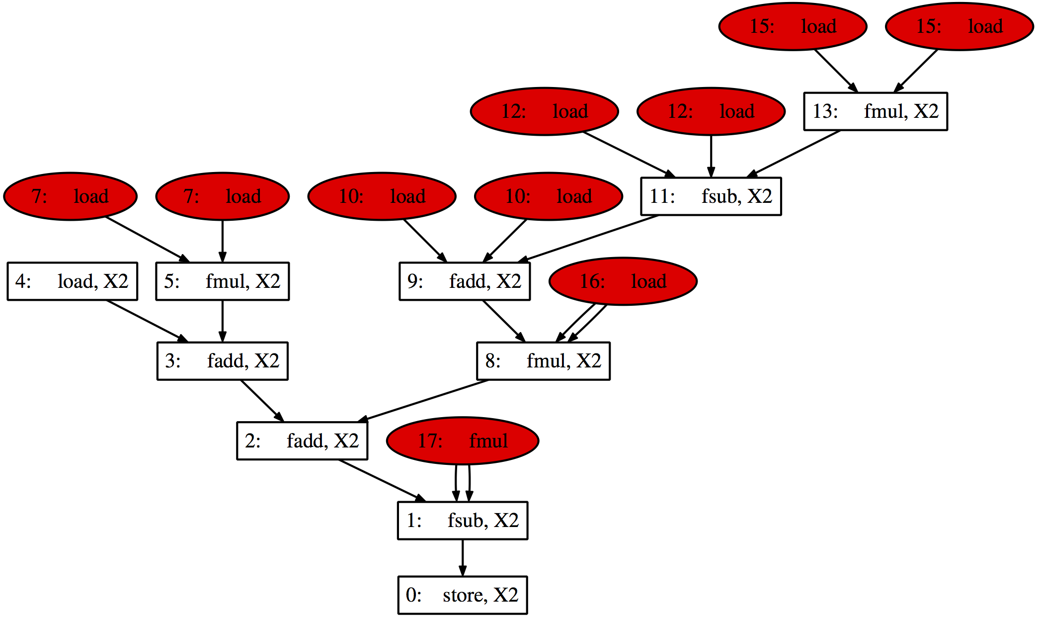
Going through the nodes, this is how they map to the code above.
- The vector subtract of lines 4 and 9 from their predecesors;
- The vector add of lines 3 and 8 with their predecessors;
- The vector add of lines 2 and 7 with their predecessors;
- The vector load of
rhs[i][j][k][2]andrhs[i][j][k][3]; - The vector multiplication of
dx3tx1with the rest of line 2 anddx4tx1with the rest of line 7; - For some reason, there is no node 6;
- These are scalar loads of globals
dx3tx1anddx4tx1, which are non-contiguous in memory, so can’t be vectorised; - The vector multiplication of
xxcon2with everything else on lines 3 and 8; - The vector add within the brackets in lines 3 and 8;
- The scalar loads of
vs[i-1]][j][k]andws[i-1][j][k]which are not contiguous in memory; - The vector subtract within the brackets in lines 3 and 8;
- The scalar loads of
vs[i+1][j][k]andws[i+1][j][k]which are, again, non-contiguous; - The vector multiplication of
2.0withvs[i][j][k]andws[i][j][k]in lines 3 and 8; - Again, no node 14;
- The actual scalar loads of
vs[i][j][k]andws[i][j][k], it’s obvious that these are non-contiguous; - The scalar load of
xxcon2, which is sent to all SIMD lanes; - The multiplication of
tx2with everything in brackets on lines 4 and 9.
Obviously node 0 is the final vector store back to rhs[i][j][k][2] and rhs[i][j][k][3] and the seed for starting vectorisation. We think the compiler has also noticed that the array u is not initialised, so lines 4 and 9 are identical.
This vectorised code results in 10 vector instructions (nodes 0-5, 8, 9, 11, 13), 10 scalar instructions (nodes 7, 10, 12, 15-17), and 10 gather instructions (1 for each of the scalar nodes; where there are two lines out of a scalar, the value is broadcast to all vector lanes, using 1 instruction). The cost model used by SLP in our case assigns a cost of 1 for each of these, leading to a total vector cost of 30. If all the code had been kept as scalar, then it would have also had a cost of 30 (each vector instruction replaces 2 scalar and there would be no gathers, so the cost is 2 * 10 + 10). This leads to no benefits from vectorisation, so the code is left as scalar.
However, looking at the graph it is easy to see that the left-hand side is vector-heavy, whereas the right-hand side has a lot of nasty red scalar instructions. These are obviously pushing up the costs of the graph, since they each have a cost of 2: 1 for the instruction and 1 for the gather we then require. We would love to remove them and see whether vectorisation is then profitable. Of course, this is what TSLP is all about.
TSLP goes through the graph considering the cost of all connected subgraphs that include the root. The following graph is the one it finds with the minimum cost, and therefore ultimately the one that is vectorised.

In this graph, the whole of the upper right-hand side, from node 8 onwards, has been kept as scalar. This means that it’s really only lines 1 & 2, and 6 & 7 that get vectorised, along with the additions and subtractions at the end of each line. The vector cost for this graph is 16 (from 6 vector instructions, 5 scalar instructions and 5 gathers), whereas the scalar cost is 17, a saving of 1. The code is inside 3 loops, each of has 10 iterations, meaning a cost saving of 1000 across the whole function, without accounting for any other code that is vectorised too. Although the amount of vector code is smaller, TSLP has ensured that the final graph is the most profitable and performance is higher than with either scalar code only or SLP vectorisation alone.